top of page


Estimation for slip ratio and adaptive control of Tracked mobile robot
Full project report:
Overview
when it comes to controlling a tracked mobile robot, the longitudinal slippage of the left and right tracks can be described by two unknown parameters. In this project, we intend to use different adaptive laws and neural network methods to estimate these slippage parameters. To compare the performance of the different estimation methods, we use Simulink and python to construct simulation models. An empirical formula of slippage was used to simulate slippage. The final results are analyzed by the the RMS value of the trajectory tracking error.
Skills & Abilities
-
Matlab / Simulink
-
Adaptive control
-
Neural Network control
-
parameter estimation
-
Trajectory tracking
Related Projects
Introduction
Recently, different applications of tracked mobile robots (TMR) are emerging more and more often in the fields of agriculture, national defense, and industry. As shown in Fig. 1, large contact areas between tracks and the ground provides better mobility in unconstructed environments. Subsequently, the problem of motion control of mobile robots becomes a popular topic among researchers. Lots of researchers have designed various tracking controllers [4] [9] [12] with the nonholonomic constraints, which is the assumption that the mobile robot are subject to a "pure-rolling without slipping" situation. However, the disadvantage of the tracks is that it increases the chance of slippage to happen in a rough terrain. Therefore, it is necessary to consider the slipping condition for mobile robots operating in complex environments. In [13], the slippage for mobile robot was categorized into lateral and longitudinal slippage. The trajectory tracking problem considering slippage was proposed in [2] and [10]. However, these studies all assume that the slippage parameters can be directly detected by the sensors in real time, which can still hardly be achieved by modern practical engineering. Hence, to compensate for the slippage, the slippage parameters must be estimated.

There are many existing researches trying to solve this problem using different approaches. The first popular approach is using adaptive law to estimate the slipping parameters [1] [7]. On the other hand, neural network are often well suited to model uncertain or nonlinear function such as mobile robot dynamics [5]. Assumed that the slippage ratio can be described by a complicated nonlinear function g(x). This time, we try to approximate the g(x) with NN.
Problem Formulation
Slippage ratio is defined as:

Where ωL and ωR are the angular velocities of the left and right wheel, r is the radius of the wheels, and vL and vR are the actual linear velocities of the wheel with slippage.
Since ωL and ωR can be measured by the encoder or any other angular velocity sensors, if we can obtain the information of vL and vR, then the slippage ratio can be directly calculated. However, there are several difficulties that impede us from doing so.
First, the nonlinear nature of the slippage parameters makes it difficult to measure the actual linear velocities of the wheel. Even if there are sensors like GPS that can obtain the information with relatively high precision, the cost of these sensors is usually unaffordable. However, using low-cost sensors to measure the linear velocities can result in magnificent noise in the signal. In addition, the low-cost sensors usually provide low sampling rate and delay, which is also a big problem when controlling the robot. Therefore, using limited information to design an adaptive law which can indirectly estimate the slippage ratio becomes a crucial topic regarding the precise control of mobile robots.
In this project, we will use different approaches to estimate the slippage ratio and compare the trajectory tracking performance.
Approaches
The kinematics of the mobile robot is defined as:
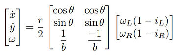
where q=[x, y, theta]^T is the Cartesian coordinate of the mobile robot, and dot{q}=[dot{x}, dot{y}, omega]^T is the time derivative of the position of the robot.
Also, r is the radius of the wheel, b is the distance between two driving wheels of the TMR. ωL and ωR are the angular velocities of the left and right driving wheels, which is controllable.
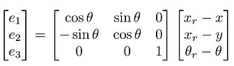
To achieve trajectory tracking, we define the tracking error e=[e1, e2, e3]^T in the global Cartesian coordinate as:
By applying backstepping control method, the auxiliary control law can be design as:
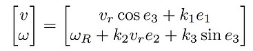
Therefore, the actual control input will be:

To calculate for the control input, we need the information of the slippage parameters.
Adaptive update law 1
For the first adaptive law, we adopted the method proposed in [1]. The adaptive law designed in this research doesn’t estimate the slippage parameters directly. Instead, the parameters were redefined as following:

The estimations of a_k are defined as hat{a}_k. On the other hand, the estimation error is defined as Bar{a}_k=hat{a}_k - a_k.
The Lyapunov function was chosen to be as following:
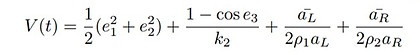
where k2, p1, p2 are positive constants.
Therefore, the adaptive law for aL and aR can be designed as the equations below to make dot{V}(t) <= 0:

Adaptive update law 2
For the second adaptive law, the method proposed in [7] was adopted. Similarly, the adaptive law designed in this research estimates the parameters defined as:
The difference is that the Lyapunov function was chosen to be as following:
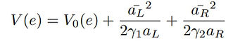
where k_2, p1, p2 are positive constants, and V0(e) is the Lyapunov function of the mobile robot tracking controller [8].
Therefore, the adaptive law for aL and aR can be designed as adaptive update law 1 to make dot{V}(t) <= 0:

Neural Network
We have introduced the application of neural network. In this paper, we try to approximate the nonlinear function g(x) and input is defined as
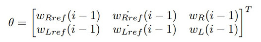
The neural network can be redefined as g(θ) : R6 → R2

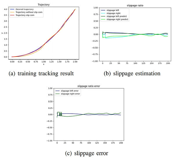
where Φ is activation function, W are weights in neural network and g is regarded as the output predicted slippage ratio [iL(i) iR(i)]T . Next we choose MLP with 6 inputs, 1 hidden layer with 10 neuron and 2 outputs, all of the layers takes the sigmoid activation function as our NN structure. Introduce the SGD as the optimizer and adopt MSE as loss function. In order to get a better performance, we train this network in the following trajectory:
Training with epochs = 200, datasets = 200 and batches = 32. The figure shows the training result. Next, we will apply this pretrained model to a different trajectory and validate it if it can accurately predict the slippage ratio. Moreover, we also introduce the online learning [6] to compare the tracking performance and slippage ratio estimation with the method of offline pretrained model.
Simulation and Discussions
After the methods have been determined, we use simulation to compare the performance for each method. To model the behavior of the vehicle, some parameters must be assumed in the simulation. The parameters of the TMR are set as follows: b = 0.15m, r = 0.075m, ζ = 1, k2 = 14, k1 = k3 = 1.
In addition, since slippage is a nonlinear behavior, using a constant to analyze the estimation performance cannot guarantee an equivalent result when implementing on the robot. Therefore, we adopted an empirical formula proposed by [11] to simulate the slippage. According to the research, the slippage parameters are exponential functions of the turning radius, which can be written as follows:

The coefficients in the formula are obtained from the average of multiple experiments. R is the radius of path and can be calculated by:

Also, to verify the effect of the estimation schemes, we increase the values of the slippage parameters by 1.3 times as much as the previous values at t = 30 sec. The block diagram of the entire trajectory tracking scheme is shown in the following figure.

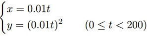
The equation of the reference trajectory is given as:

where t ≥ 0 is the simulation time. The initial posture of the reference trajectory is set at:
However, to demonstrate the tracking ability, the actual initial posture of the TMR is set at:
Adaptive laws
The initial conditions are chosen as ˆaL(0) = ˆaR(0) = 1. Also, the estimation gains are set to be ρ1 = ρ2 = 5, γ1 = γ2 = 50. The results of the first adaptive law can be seen in the figures below:

We can see that the estimation errors of the parameters quickly reduce to about 0.04 within 10 secs. However, with the change of the angular velocity of the two wheels, the slippage ratios also change. The convergence of the estimation couldn’t keep up with the sudden change of the parameters, resulting in a rising of the estimation errors. Moreover, when the slippage ratio suddenly magnifies at t = 30, the estimation errors rise again. The final estimation error when t = 81 is ¯iL = 0.1253, ¯iR = 0.0669
For the second adaptive law we adopted, the results are in the following figures:

From the results, we can see the convergence happens faster than the first adaptive law. The estimation errors reduced to < 0.001 within 8 secs. However, when the parameters increase at t = 30, the changes in the estimations are inapparent. Nonetheless, the estimation performance is still better than the first adaptive law. The final estimation error when t = 81 is ¯iL = 0.02398, ¯iR = 0.01026
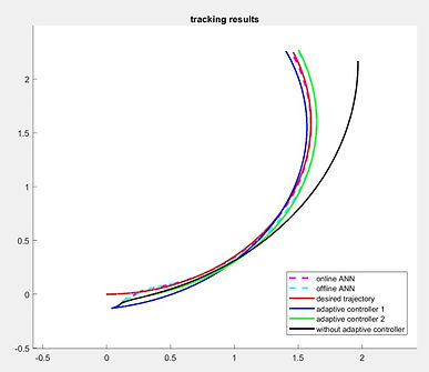
The figure below demonstrates the trajectory tracking results of the TMR using the two different adaptive laws. To distinguish the effect after compensating for the slippage, the tracking result without using the adaptive controller was also in the figure.

From the tracking result, it is clear that with the implementation of adaptive controller, the negative effect of the slippage can be canceled, which greatly benefits the tracking performance. On the other hand, the difference between the two trajectories using different adaptive laws are not very obvious. The figure below shows the tracking error along the reference trajectory.

Since the convergence rate using the first adaptive law is slower, the result using it has more error at the beginning. Therefore, despite the insignificant difference, we can still suggest that the tracking ability using the second adaptive law are slightly better.
Neural Network
Uniform slippage ratio
We choose python and ML tool box, keras as our simulation platform to construct the neural network model.
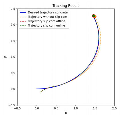
1) The slippage ratio remains the same: In the figure above, the result shows that the tracking performance with the offline NN slippage compensator is better than that without the compensator. However, because the NN training data is not from this desired trajectory, the offline tracking trajectory is not as good as the online tracking trajectory.
2) The slippage ratio changes when t > 30sec: In this case, the defect of the offline NN slippage compensator reveals, which is that us cannot catch the desired trajectory. By contrast, tracking with online NN compensator almost overlaps with the desired trajectory in the figure below.
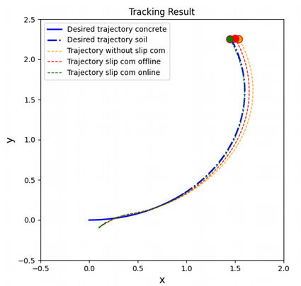
Slippage ratio changes when t > 30s
The following figure shows the comparison of slippage ratio estimation and estimation error between online and offline NN compensator. Online NN compensator has smaller slippage ratio error and better slippage tracking performance.

3) offline v.s. online: We can regard the changing in the slippage ratio as the different terrain or soil condition the TMR robot encounters in the real world. A lot of factors that affect the slippage ratio we won’t know in the future. Therefore we need online learning to update the slippage compensator model in time.
Neural Network vs adaptive

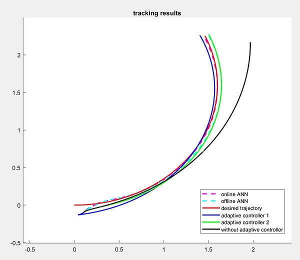
The figure above shows the tracking result of the four compensator methods. All of the four methods effectively predict the slippage ratio. To evaluate which method come to a best tracking performance. We introduce RMS value of tracking error as criterion

we define


RMS value of four slippage compensator
The following figure shows the error of x, y and θ along the tracking process and Table I shows the RMS value of four slippage compensator methods.
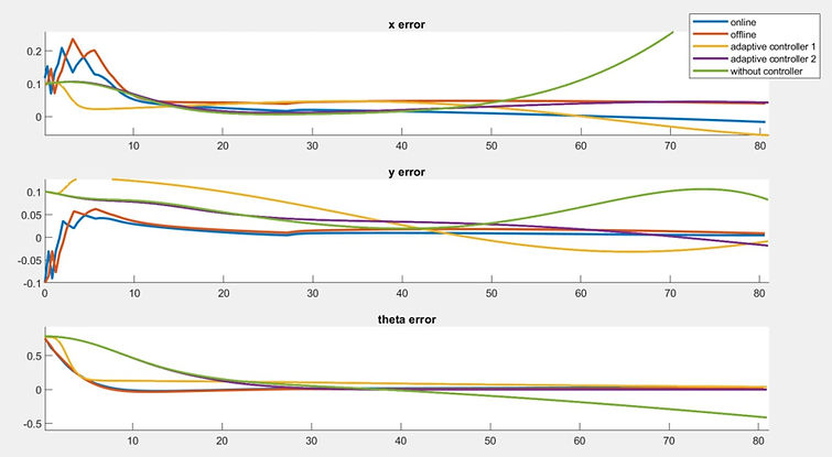
Only offline NN compensator has larger RMS, and the other three compensators have outstanding performance.
Conclusion
In this paper, we describe how difficult to model the slippage ratio and how slippage ratio have an impact on tracking trajectory. To deal with the problem of slippage ratio, we introduce two methods of adaptive designs and online/offline neural network to estimate the slippage ratio. Finally, we prove that we can predict the slippage ratio correctly and enhance tracking performance by matlab and python simulation. Next, we simulate these slippage-ratiopredicted methods on various trajectories to validate its robustness. Finally, we will implement it on a real TMR robot.
References
[1] Mingyue Cui. Observer-based adaptive tracking control of wheeled mobile robots with unknown slipping parameters. IEEE Access, 7:169646–169655, 2019.
[2] Mingyue Cui, Rongjie Huang, Hongzhao Liu, Xuyan Liu, and Dihua Sun. Adaptive tracking control of wheeled mobile robots with unknown longitudinal and lateral slipping parameters. Nonlinear Dynamics, 78(3):1811–1826, 2014.
[3] Mingyue Cui, Hongzhao Liu, Wei Liu, and Yi Qin. An adaptive unscented kalman filter-based controller for simultaneous obstacle avoidance and tracking of wheeled mobile robots with unknown slipping parameters. Journal of Intelligent & Robotic Systems, 92(3):489– 504, 2018.
[4] Mingyue Cui, Wei Liu, Hongzhao Liu, Hualong Jiang, and Zhipeng Wang. Extended state observer-based adaptive sliding mode control of differential-driving mobile robot with uncertainties. Nonlinear Dynamics, 83(1-2):667–683, 2016.
[5] Haibo Gao, Xingguo Song, Liang Ding, Kerui Xia, Nan Li, and Zongquan Deng. Adaptive motion control of wheeled mobile robot with unknown slippage. International Journal of Control, 87(8):1513– 1522, 2014.
[6] Steven C. H. Hoi, Doyen Sahoo, Jing Lu, and Peilin Zhao. Online learning: A comprehensive survey, 2018.
[7] Juliano G Iossaqui, Juan F Camino, and Douglas E Zampieri. A nonlinear control design for tracked robots with longitudinal slip. IFAC Proceedings Volumes, 44(1):5932–5937, 2011.
[8] Doh-Hyun Kim and Jun-Ho Oh. Globally asymptotically stable tracking control of mobile robots. In Proceedings of the 1998 IEEE International Conference on Control Applications (Cat. No. 98CH36104), volume 2, pages 1297–1301. IEEE, 1998.
[9] Yongfu Li, Chuancong Tang, Srinivas Peeta, and Yibing Wang. Integral-sliding-mode braking control for a connected vehicle platoon: theory and application. IEEE Transactions on Industrial Electronics, 66(6):4618–4628, 2018.
[10] Chang Boon Low and Danwei Wang. Gps-based path following control for a car-like wheeled mobile robot with skidding and slipping. IEEE Transactions on control systems technology, 16(2):340–347, 2008.
[11] S Ali A Moosavian and Arash Kalantari. Experimental slip estimation for exact kinematics modeling and control of a tracked mobile robot. In 2008 IEEE/RSJ International Conference on Intelligent Robots and Systems, pages 95–100. IEEE, 2008.
[12] Luy Nguyen Tan. Omnidirectional-vision-based distributed optimal tracking control for mobile multirobot systems with kinematic and dynamic disturbance rejection. IEEE Transactions on Industrial Electronics, 65(7):5693–5703, 2017.
[13] Danwei Wang and Chang Boon Low. Modeling and analysis of skidding and slipping in wheeled mobile robots: Control design perspective. IEEE Transactions on Robotics, 24(3):676–687, 2008
bottom of page