
Digital controller implementation for Tracked mobile robot
Overview
In this project, we first use system identification to estimate the transfer function of the motor with different sampling times. Then, we compare the models and find a particular model can be approximated with a first order system. Next, we use pole placement method to decide the gains for the PI controller. Using common digital PI controller approximations, we turned the continuous-time controller into a discrete controller. By comparing the step responses, we verified the performance of the digital controller acting on different estimated models. After confirming the specifications are all satisfied, we implemented the digital controller on the actuator. In addition, to avoid integral windup, we also implemented anti-windup features in the controller.
Finally, to analyze the influence of the controller on trajectory tracking control, we use Simulink to compare the results.
The results suggest that, by implementing the digital PI controller, the trajectory tracking ability of the TMR was improved.
Skills & Abilities
-
Matlab / Simulink
-
System Identification
-
Pole placement
-
Digital PI controller implementation
-
Anti-windup compensation
-
Trajectory tracking
Related Projects
Systems
A tea harvesting robot has been developed to reduce the workload for farmers and resolve the labor shortage problem in Taiwan. The robot is designed to be a Tracked Mobile Robot (TMR).
To maintain a stable movement and adapt in various terrain conditions in agricultural fields, we designed the vehicle to be a tracked mobile robot. Large contact area between tracks and the ground provides better mobility in unconstructed environments. However, the disadvantage of the tracks is that it increases the friction between the tracks and the ground, which can have a negative effect for the motors to track their reference angular velocities. Therefore, digital controllers are required to solve this problem.
In this project, we will develop a digital angular velocity controller and try to implement it on the TMR. Also, we will use simulations to compare the trajectory tracking ability with or without the controller.

The block diagram of the tracked mobile robot can be demonstrated by the figure above. The subsystem of the motors is a crucial part regarding the trajectory tracking ability of the TMR.
Thus, designing a controller satisfying the specifications can be a vital problem to increase the tracking performance of the robot.
The kinematic model for the mobile robot can be derived as following:
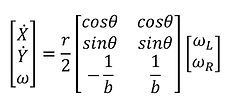
Therefore, by controlling the angular velocities of the two motors, we can control the linear and angular velocities of the robot on a 2D plane.
Controller design specification
-
Overshoot < 5 %
-
Settling time < 2 secs
-
Steady-state error < 1 %
Modeling
To identify our motor model, a black box test is implemented. We treated our motor plant model as a black box in an open-loop system, given step and sin-wave with different frequencies as input duty cycle and use encoder to collect the output angular speed with different sampling time.
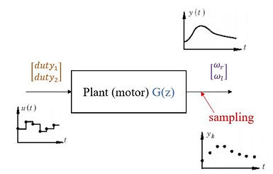

For different input sequence, we choose step function and sin wave to discuss the difference between each estimated model with different input signals. Also, to further discuss the influence of the different input sin-wave frequencies, we tested three different kinds of frequencies and measured their output.
For different sampling time, we choose Ts=0.01s, Ts=0.05s, and Ts=0.1s to discuss the difference between each model with different sampling time.
After multiple experiments, we collected different output data and preprocess them before putting them into the system identification toolbox.

System Identification toolbox (Matlab)

The system identification toolbox in Matlab is used to construct mathematical models of dynamic systems from measured input-output data. Therefore, we can estimate the transfer functions of each data and validate them using different datasets.
When estimating the transfer functions, we assumed the number of poles to be 2 and the number of zeros to be 1.
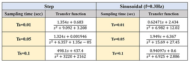
The table below shows the estimated transfer functions with different sampling time and different input sequence.
Analysis
Pole-zero maps

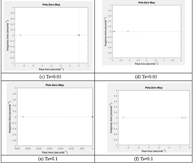
From the pole-zero maps, we can see a trend that for the models obtained from sinusoidal responses, with the increase in sampling time, the dominant poles are getting closer and closer to the origin.
Also, for the models obtained from step responses, the model with Ts=0.05 has one RHP zero, which means the system is a nonminimum phase system, which can cause a phase lag on the system.
To compare the difference between the models and to validate the approximation accuracy of each model, we use a different set of data obtain through experiment with a sampling time of Ts =0.05 to treat as a validation data.

We can see that all of the models have similar step responses. Therefore, choosing a model with the lowest order after pole-zero cancelation can reduce the complexity of the designing problem. Since the model obtained through sinusoidal response with a sampling time of Ts=0.01 has a zero and pole very close to each other, we can approximate the model with a reduced order system.
The pole-zero cancelation process is shown below.

Controller design
A typical digital controller design process can be categorized into two kinds of method. You can either directly design a digital controller from a discrete-plant, or you can first design a continuous-time controller and using an approximation to convert the CT controller into a DT controller. The former method is called the Discrete design, whereas the latter method is called Emulation.

Putting the zero between the poles can result in a slow closed-loop response. If the zero is placed to the left of the open-loop pole, the closed-loop response can be faster than the open-loop response (the closed-loop poles can be closer to the origin).
However, since the closed-loop poles can be complex, there could be overshoot in the closed-loop response, which may be undesirable.
From the figures, we can see that despite a little overshoot, the settling time for the zero placing at the left of the poles is much faster than that at between the poles. Therefore, to meet our requirement, the zero was chosen to place at z=4.3761. Also, K was chosen to be 5.2773 to have the best transient response while meeting our design criteria. As a result, the gains can be computed as follows:

While the PI controller can be written as:

where Kp and Ki are the controller gains to be determined.
Therefore, to decide the values for , we can use the pole placement method.
First, the open loop transfer function can be reduced to:

Where K = 0.6247 Kp and z = Ki/Kp
With the open loop transfer function, we can now decide where the zero can be placed.
Since the open loop poles are located at s=0 and s=3.087, we can place the zero at either between the poles or left of both the poles. The two pole placement choices and their step responses are shown below.
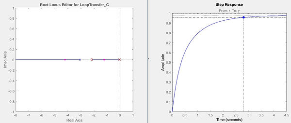
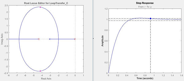
Putting the zero between the poles can result in a slow closed-loop response. If the zero is placed to the left of the open-loop pole, the closed-loop response can be faster than the open-loop response (the closed-loop poles can be closer to the origin).
However, since the closed-loop poles can be complex, there could be overshoot in the closed-loop response, which may be undesirable.
From the figures, we can see that despite a little overshoot, the settling time for the zero placing at the left of the poles is much faster than that at between the poles. Therefore, to meet our requirement, the zero was chosen to place at z=4.3761. Also, K was chosen to be 5.2773 to have the best transient response while meeting our design criteria. As a result, the gains can be computed as follows:

Therefore, the result of the controller implementing on the original plant is shown below.

After the continuous-time controller has been established and verified, we can now discretize the controller.
A common approximation of the digital PI controller is shown below:

Therefore, by substituting the values for Kp and Ki obtained from the previous section, D(z) can be computed as:

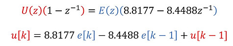
However, to implement the digital controller, it would be necessary to express the transfer function with since the input sequence needs to be causal.

In addition, deriving the transfer function into a difference equation can make the implementation more intuitive.
Next, we implement the digital controller on models established by different sampling times to verify the performance of the controller remains unaffected.
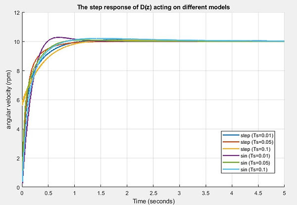
We can see that the effect of the controller is unanimous across different models established with different sampling time and different input frequencies. The only overshoot in the responses is occurred in the original plant, which is 2.93%, satisfying the requirement. Also, not only all of the responses have no steady-state error, the settling times are also less than 2 secs.
Since all of the design criteria has been fulfilled, the controller can now be implemented on the actuator to analyze the result.
Implementation and Results
A typical problem when implementing the PI controller on an actuator is the saturation and integral windup.
This problem is caused by a limited output of a physical system. For instance, when the error between the reference and the output of the system is large, it can result in a control input greater than the system can accept. As a result, the output of the system is smaller than expected, causing error to be integrated. When the output finally reaches the reference, the errors had been accumulated so much that the integral action can become larger than the system needs. Consequently, the controller will create a huge overshoot at the output until the integrator is discharged.
Therefore, to avoid this problem, an anti-windup compensation is necessary when implementing a PI controller.
The general idea for an anti-windup controller is that when the actual output and the expected output are not equal, the integrator will be turned off. The error will not be accumulated once the system becomes saturated.
This mechanism is realized by making the comparison between the actual output and the expected output become the on-off switch of the integrator.

The following code was the digital PI controller written in C language.

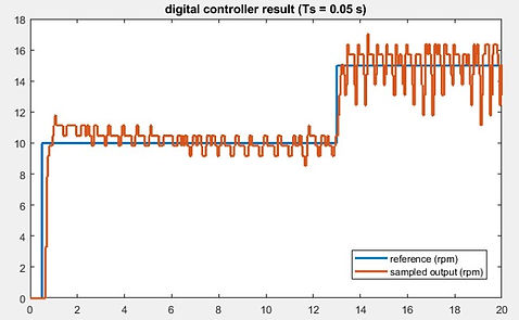
After implementing the digital controller into a program, we can test it on the tracked mobile robot (TMR) and see the result.
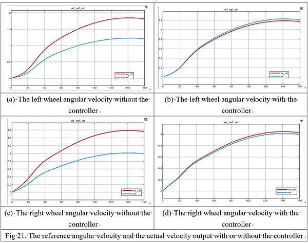
The result of the angular velocity control of the motors on the TMR can be seen in the following figure.

The reference angular velocity was set to be a step input, where:

The sampling time was set to be Ts=0.05s.
We can see that after the reference changes at t=0.5, it was not until t=0.65 that the sampled value starts to change. This delay can be caused by many reasons:
-
The calculation delay of the computer
-
The input delay of the control card
-
The delay from the encoder
-
The sampling delay
At the first step reference, after the output approaches the reference, it overshoots for an average of 11.3%. Ignoring the noises, the overshoot is still higher than expected. However, the sampled output tracks the reference with a steady performance. The transient response of the system are quick and the rise time and settling time are small enough.
The second step occurs at . This time, the overshoot is inapparent. Also, the delay is smaller and the transient response are better.
Simulation
In this section, we will use Simulink to construct a simulation model to verify the performance of the digital control and its influence on the trajectory tracking ability.
To model the behavior of the vehicle, some parameters must be assumed in the simulation.
The reference trajectory was set to be a circular trajectory, where:

The initial position of the reference trajectory qr(0) and the robot q(0) are:
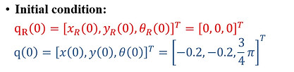
The initial position of the robot was set to be off the reference trajectory to inspect the performance of the controller.

The following is the trajectory tracking control scheme:
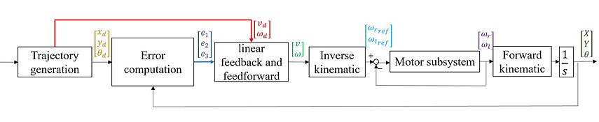
Thus, the Simulink model can be constructed as the following:

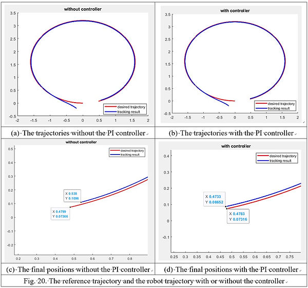
The trajectory tracking results can be seen below.
Although the differences between the tracking result is not very obvious, we can still see a improvement of tracking ability when the digital controller was implemented.
(c) and (d) is the zoom in figures on the final positions. We can see that the final position of the robot is deviated from the reference final point for an error of xe=0.0581m, ye=0.03594m without the controller.
However, the error was reduced to xe=0.005m, ye=0.01336m, which can greatly benefit the tracking ability.