Autonomous Forklift

263498853_507833413725842_1168043400876210076_n_edited.jpg

Autonomous Forklift

Overview

To alleviate the high demand for laborers, Coretronics robotics Corporation had developed an autonomous forklift. I was honored to join this project as a intern. My goal in this project was to research and implement a second-order derivative continuous path planning algorithm on the autonomous forklift. After researched on numerous papers, I finally decided to implement the Double Continuous Curvature (DCC) path planning algorithm in the simulation.

Apart from the imperative coding skills I developed via constructing a path planning simulation for an autonomous forklift using Matlab and Simulink, I also learned about the importance of business concepts in the industry. To become a competent robotics engineer, identifying market requirements, and managing a team are just as crucial as the technical abilities we learnt in school. Therefore, this experience inspired me to continue my studies and pursue a career in this field.

Skills & Abilities

Matlab and Simulink
Programming (C++)
Path planning algorithms
System Identification

Requirements

1. Conduct system identification on the forklift and use the data in the simulation
2. Simulate the movement of the autonomous forklift using 2D graphic interface
3. Implement various path planning algorithm on the simulation and analyze the feasibility and error.

Kinematic model

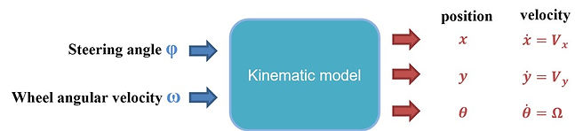
The forklift is consist of three wheels. The wheel at the front is the steering wheel, we can only control its steering angle. The two wheels behind are the driving wheels, whose angular velocities are controllable.
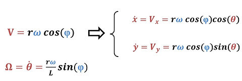
To simulate its movement, we first need to derive its kinematic models. Then, we can use the equations to determine its coordinate in the 2D plane.

System Identification

To model the system behavior as similar to the reality as possible, I conducted a system identification for the actuators on the forklift. The input and output data are shown in the figures below. Then, I used these data to identify the transfer function of the motors.

Overshoot 37.5%

Delay 0.33 sec

Rise time 1.37 sec

wheel velocity step response data

Overshoot 14.28%

Settling time 0.79 sec

Accuracy within 0.5 deg

steering angle step response data

Simulation model

Using Simulink, the simulation model was created. This simulation can visualize the 2D movement of the forklift taking the real behavior of the actuator into consideration. The red box on the left is the control panel, which allows users to change the velocity and steering angle of the forklift. Then, through the kinematic model derived above, we can convert the velocity and steering angle to coordinates visualize it on a plot.

Path planning algorithms

The goal is to find a path planning algorithm that can generate a second-order derivative continuous shortest path to the destination. There are various kinds of path planning algorithms, which can be seen in the following.

The simplest path planning algorithms are the "Dubins curve" and "Reeds and Shepp curve", which only consist of circular path and linear path. The only difference is that Dubins curve only allows the object to move forward, while the Reeds and Shepp curve allows the object to move backwards. However, these kinds of paths are not second-order derivative continuous, which means it will not generate a smooth path for the robot to follow. The curvature of this type of path is discontinuous so that if a car-like robot were to actually follow such a path, it would have to stop at each curvature discontinuity so as to reorient its front wheels.

Dubins curve

Reeds and Shepp curve

Another types of curves are the continuous curvature curves. For example, the "elementary" and "Bi-elementary" paths shown below. These paths are made up of clothoid arcs, whose curvature is a linear function of their arc length. The loci of the intermediate configuration is restricted to a circle with specific orientations to ensure that each Elementary path contains symmetrical clothoids. Therefore, the downside of these types of curves is that the solution space is limited, making them unsuitable for object avoidance.

Elementary path

Bi-elementary path

A Single Continuous-Curvature path (SCC) simplify the problem of finding optimal path. Each path is defined as the combination of a maximum of 7 parts between clothoids, circular arcs and line segments. As shown therein after SCC-paths can only cope with a limited set of solutions. For this reason, SCC-paths will be only used as a basis of Double Continuous-Curvature paths (DCC). DCC paths use two SCC paths to provide a set of general solutions. The figures below demonstrates the difference between these paths and their curvature profiles. The DCC path is suitable for planning the path for the forklift due to its continuous curvature profile and wider range of solution space. As a result, I decided to adopt DCC path planning algorithm and try to implement it in the simulation.

Double Continuous Curvature (DCC) path

To implement the algorithm, we need to define the formulas for the DCC path. The formulas to calculate for each section of the path can be seen below. qA is the starting pose, while qB is the destination.

The Clothoid part of the curve, which is the part where the curvature is changing as a linear function of its length, uses Fresnel integral to calculate its x and y coordinate. The calculation can be seen in the equations below.

When planning the path for a vehicle, we need to consider that the curvature of the starting position might not be 0, which means the steering angle of the vehicle might not be 0. As a result, the first section of the DCC path might not be a straight line, but starting from the Clothoid section. The same thing can be applied to the ending part of DCC paths.

After using Fresnel Integral to solve for the x, y, theta within each clothoid, the following equations can be used to solve for l_A, l_c, and theta_c.

Implementation

After spending weeks trying to figure out the formulas, I used Matlab to implement the algorithm. The flow chart of the algorithm is shown above. The algorithm was able to generate a DCC path and plot the results after specifying the starting and ending position. If I specify the starting point q_A = [0, 0, 1, 0], and the destination q_B = [0.7, 0.5, pi/2, 0], then it will automatically generate a smooth path. The results can be seen below. The curvature profile demonstrates the continuity of the second-order derivative of the path, indicating the smoothness of the path satisfies the requirement.

Curvature profile

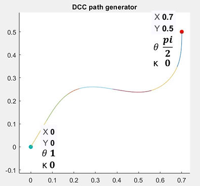
DCC path generation

Path planning simulation

[Path planning simulation]

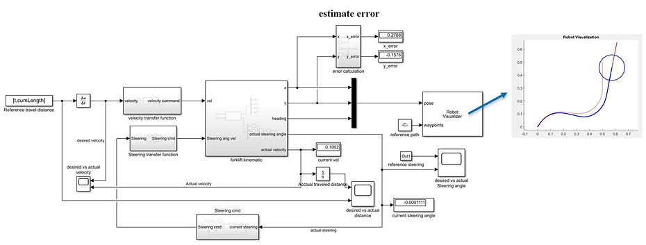
After successfully implemented the path planning algorithm on matlab, I then used Simulink to integrate the algorithm and the simulator I constructed. With this integration, the real behavior of the forklift can be taken into consideration. Consequently, I can analyze the error of the algorithm using this simulation before applying it on the forklift.

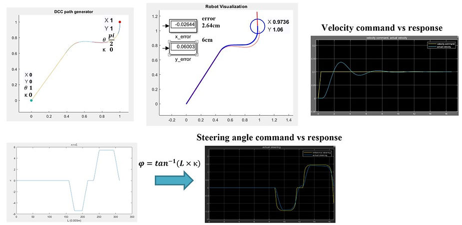
In the simulation results, we can see that the vehicle was able to track the generated path with an acceptable amount of position error. This error may be caused by the velocity response during the start of the trajectory. However, this is because I didn't design any trajectory tracking controller in this project. Therefore, if the controller was added, it can improve the performance of the velocity and steering angle responses. This way, the tracking ability can be improved, and the error will reduce significantly.

Conclusion and Future work

In this project, an autonomous forklift was developed. To be able to move smoothly, a Double Continuous Curvature path planning algorithm was implemented in the simulation. System identification was used to model the behavior of the forklift. The final result was analyzed comparing the expected results to the model gained from system identification.

For future work, trajectory tracking controller was needed to reduce the tracking error. Additionally, real time calculation to generate the path would be essential to plan for the intermediate way points. This way, the forklift can fix its direction between each waypoint, and the final position error can be further reduced.

Supplementary Materials

Taipei International Industrial Automation Exhibition 2020

During the last day of my internship, I was given the opportunity to attend the 2020 Taiwan International Industrial Automation Exhibition. The picture on the right is our stall at the exhibition. I co-worked with my colleagues to promote the autonomous forklift during the event. In this event, I was able to learn about how to
communicate with the customers and address their needs. In addition, whenever there was any unexpected issues, I can identify them quickly and handle them prudentially.

[our stall at the exhibition]

This experience not only enables me to take a glance of the state-of-the-art automation technology in the industry, I also realized the importance of marketing concepts.

[me and my colleagues]

References

[1] Girbés, Vicent, Leopoldo Armesto, and Josep Tornero. "Path following hybrid control for vehicle stability applied to industrial forklifts." Robotics and Autonomous Systems 62.6 (2014): 910-922.

[2] Girbés, Vicent, Leopoldo Armesto, and Josep Tornero. "Continuous-curvature control of mobile robots with constrained kinematics." IFAC Proceedings Volumes 44.1 (2011): 3503-3508.

[3] Girbés, Vicent, et al. "Continuous-curvature kinematic control for path following problems." 2011 IEEE/RSJ International Conference on Intelligent Robots and Systems. IEEE, 2011.

[4] Espinosa, Felipe, et al. "Modelling and Simulation of the Kinematic and Dynamic Behavior of a Fork-Lift-Truck." IFAC Proceedings Volumes 31.3 (1998): 51-55.